Understanding Lagrange Multiplier, KKT Condition and Dual Problem
Why Lagrange multiplier \(\lambda\) can work
Let’s consider general multi-dimensional constrained optimization problems. To find the optimized point, one can start from where the constraint is satisfied. Every constraint can be viewed as a hyper-surface (including point and curve), where at each point allowable moving directions \(A\) must be orthogonal to local gradient to go along the contour.
\[C(x)=0, ~ A = (\nabla C(x))^{\bot}\]Taking all constraints into consideration, allowable directions for modifying \(x\) to change the optimized term is:
\[A = (\nabla C_1)^{\bot} \cap (\nabla C_2)^{\bot} \cap \dots \cap (\nabla C_n)^{\bot}.\]If this is the optimized point, the gradient of term to be optimized (max or min) mustn’t lie in this allowable space. Otherwise, the term can be further optimized without violating all constraints.
\[\nabla f(x) \in \bigg((\nabla C_1)^{\bot} \cap (\nabla C_2)^{\bot} \cap \dots \cap (\nabla C_n)^{\bot} \bigg)^{\bot}\]This is equivalent to:
\[\begin{aligned} \nabla f(x) &\in Space\{\nabla C_1,\nabla C_2,\dots,\nabla C_n\} \\ ~~~~~~~~~~~~~~~~~~~~~~~~~~~~~~~~~~~~~~~~ \Rightarrow \nabla f(x) &= \lambda_1 \nabla C_1+\lambda_2\nabla C_2+\dots+\lambda_n\nabla C_n ~~~~~~~~~~~~~~~~~~~~~~~~~~~~~~~~~~~~~(1) \end{aligned}\]This explains why in Lagrange Multiplier, constructing higher dimensional \(L\) space can resolve the problem:
\[\begin{aligned} L &= f(x)-\sum_i^n \lambda_i C_i(x)\\ \nabla L =0&=\nabla f(x) - \lambda_1 \nabla C_1-\lambda_2\nabla C_2-\dots-\lambda_n\nabla C_n ~~~~~~~~~\dots\dots explained~as~(1)\\ with& ~~~ C_i(x)=0 ,~i=1\cdots n~~~~~~~~~~~~~~~~~~\dots\dots\dots\dots constraint~hypersurfaces \end{aligned}\]Here, the sign of \(\lambda\) cannot be quite informative for equality constraints. However, it can provide some foresight for inequailty constraints.
KKT Conditions for Inequality Constraints
If one constraint is \(c(x) \leq 0\), it would be equivalent to \(c(x) + p_1^2 = 0\).
If one constraint is \(c(x) \geq 0\), it would be equivalent to \(c(x) - p_2^2 = 0\).
Here, \(p\) can be any number, and thus treated as additional dimensions together with \(x\). Therefore, one can obtain the relation of (1) for \(p_j\) dimension as:
which means either \(\lambda_j\) or \(p_j\) is 0. If both are 0, it means the equality case of this constraint is useless. However, this happens only if you provide an useless constraint (like other provided constraints already satisfy this constraint).
In this scenario, only \(\lambda_j = 0\) and \(p_i \neq 0\) holds. No need at all to consider if both are 0, and \(\lambda_j \neq 0\) with \(p_i = 0\) would yield no solution. In general, we only consider one of \(\lambda\) and \(p\) is 0, to see if a valid solution can be derived.
Another important feature for inequailty constraint optimization is, signs of \(\lambda\) can be infered under good conditions. That is because when letting \(\nabla L = 0\), we are indeed finding extrema of \(L\).
From KKT, constraints are actived only when equality, where \(\frac{C(x')}{||C(x')||}\nabla C\) (\(x'\) is an inequailty position) is the normal direction not violating the constraint. Moving towards such direction, the point is no longer extrema, but \(f(x)\) may be further optimized if the orginal extrema dose not give global maximum or minimum. Just find an extrema dose not guarantee the final optimal solution.We can, however, save part of the comparison by determining signs of multipliers.
For each constraint, if \(f(x)\) is to be maxmized, the sign of \(-\lambda C(x)\) should be positive:
On constraint hyper-surface, \(\nabla f\) is the direction in which \(f(x)\) increases, which should be opposite (just normal component of \(\nabla f\) with respect to the constraint hypersurface) to \(\frac{C(x')}{||C(x')||}\nabla C\) only in which the constraint is satisfied, if it is the optimal point. So you don’t find further increase of \(f(x)\) within the constraint.
For each constraint, if \(f(x)\) is to be minimized, the sign of \(-\lambda C(x)\) should be negative:
On constraint hyper-surface, \(-\nabla f\) is the direction in which \(f(x)\) decreases, which should be opposite (just normal component of \(\nabla f\) with respect to the constraint hypersurface) to \(\frac{C(x')}{||C(x')||}\nabla C\) only in which the constraint is satisfied, if it is the optimal point. So you don’t find further decrease of \(f(x)\) within the constraint.
However, we have many constraints, so it is a combined effect. If you know more features about the constraint functions and optimization function, a clearer sign might be concluded.
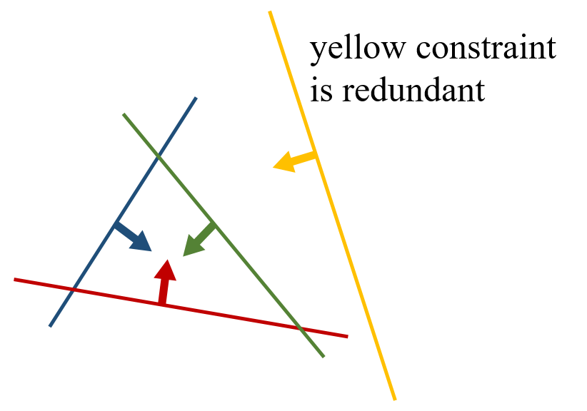
For example, let’s consider a well-defined situation where we can indeed determine the sign of each \(\lambda\). If the optimized term \(f(x)\) is a \(L2\) norm \(||\sum x_i^2||\), whether miximized or minimized, it can construct a high-dimension sphere in Euclidean space. Suppose every constraint is a high-dimension linear plane \(\sum w_i x_i+b=0\), then good things come. That is, when dealing each constraint individually, \(\nabla f\) is parallel to \(\nabla C\) to be the extrema, and \(\frac{C(x')}{||C(x')||}\nabla C\) must have different sign with \(\nabla f\) if maxmized and \(-\nabla f\) if minimized, Just as stated before. However, in such scenario, even we combine all constraints, at optimal point, \(\nabla f\) is still the linear combination of each individual base direction, where the sign of each cannot be changed. This is because, high-dimension linear plane has uniform gradient direction, so you don’t need to change \(\nabla C\) from individual situation to golobal optimal point. Additionally, a sphere is convex everywhere (only positive weights from different directions for a middle position; why the optimal is in middle of individual positions? because for a sphere and linear planes, the intersection of intersectable planes must correspond to the pointing in middel of individual tagential positions!), so when doing linear combination, you should never change the sign of each base vector regardless of sphere radius change, at most you multiply with 0 for equality constraint not activated here. Observing these properties, construct from individual extremas to global extrema would be more informative. Below is a simple example.
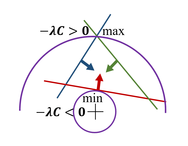
In above illustration figure, the same constraints can yield two extremas of \(L\). Depending on whether it is \(\max f(x)\) or \(\min f(x)\), the sign of \(\lambda\) is different, so as the final solution.
Sometimes, you still need to compare multiple extremas even signs of multiplier are determined.Of course you can solve for both signs of \(\lambda\) and compare each \(f(x)\) magnitude, but if you can actually know the sign like above case, why not save part of the calculation?
Now, signs of \(C(x)\) are known from the constraints, so we can determine signs of corresponding \(\lambda\). There’s another intuitive but not rigorous derivation. In each above case, obtaining extrema of \(L\) encourages either to violate constraints or not to optimize \(f(x)\), but not to acheive both we want.
Dual Problem for Lagrange Multiplier
Suppose we want to maximize \(f(x)\) with constraints \(C(x)\) and denote the solution as \(x^*\), then we know \(\max L(x) \geq L(x^*)\). If just like previous \(L^2\) norm optimization and linear hyper-planes, the sign of \(L(x)-f(x)=-\sum \lambda_iC(x)\) must also be positive signs. It then has \(\max L(x) \geq L(x^*) \geq f(x^*)\). The dual problem is designed to simplify the orignal optimization, the constraint of \(C(x)\) is sometimes tedious to process especially for multi-combinations of inequailty constraints (judge of 0 for \(\lambda_i\) and \(C_i(x)\)). Therefore, if we get the relation of \(\lambda\) and \(x\) by resolving \(\max L(x,\lambda)\), we can define \(\max L(x,\lambda)\) solely as \(q(\lambda)\). Indeed, the constraint \(C(x)\) can be violated if \(\lambda\) is not constrained from its relation with \(x\) and \(C(x)\). But it doesn’t matter, as it is always \(q(\lambda) \geq f(x^*)\) no matter what the \(\lambda\) is. So if we have \(\min q(\lambda)\) with the solution \(\lambda^*\). And if under Slater Condition, one can indeed has \(q(\lambda^*)=f(x^*)\), so here \(\lambda^*\) derives \(x^*\) and vice versa. Thus, both the dual problem and orignal problem are simultaneously solved.
In conclusion, \(q(\lambda)\geq q(\lambda^*)\geq f(x^*) \geq f(x)\).
If \(q(\lambda^*) = f(x^*)\), \(\min q(\lambda) = \min_\lambda \big( \max_x L(x,\lambda)\big)\) is the strong dual problem. And solving this dual problem gives the same solution as the orginal one.
If \(q(\lambda^*) > f(x^*)\), \(\min q(\lambda) = \min_\lambda \big( \max_x L(x,\lambda)\big)\) is the weak dual problem. Solving this dual problem gives an approximate or slack solution for the orginal one.
From my point of view, whether this “=” can hold or not should depend on whether the original constraint \(C(x)\) can be maintained at \(\lambda^*\) with corresponding \(x\).
Lagrange Multiplier and Dual Porblem also have much evidence in SVM for machine learning, a reference can be found here.